
- To clear formatting, highlight the cells. Click "Home" → "Clear" → "Clear Formats".
- For conditional formatting, highlight the cells. Click "Conditional Formatting" → "Clear Rules" → "Clear Rules from Selected Cells".
- Add "Clear Formats" to the Quick Access Toolbar or the ribbon in "Options".
Clearing Formatting

Open a project in Microsoft Excel. You can use an existing project or create a new spreadsheet. Microsoft Excel is available on Windows and Mac. You can also use the online web version at the Microsoft 365 website. You can use Excel to make tables, type formulas, make graphs, and more.
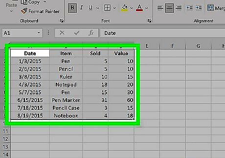
Highlight the cells you want to change. You can click and drag to select the cells. To select all, press CTRL + A (Windows) or Command + A. To select a column or row, click the column or row heading. To select specific cells, hold CTRL (Windows) or Command (Mac) and click the cells you want to select.
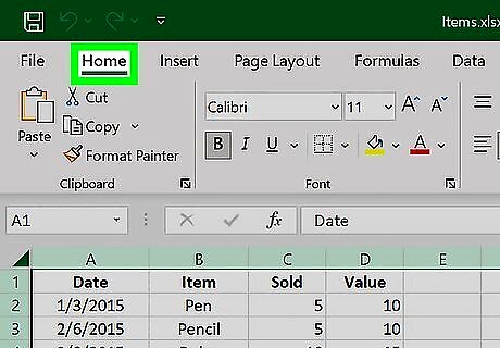
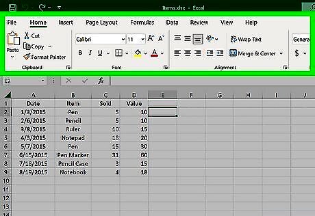
Click Home. You can find this on the top toolbar, next to Insert. You may already be on this tab.
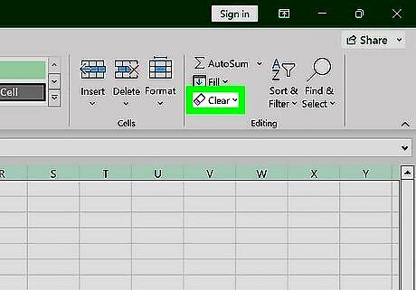
Click Clear. This will be in the Editing section on the right side, next to an eraser icon. A dropdown menu will open.
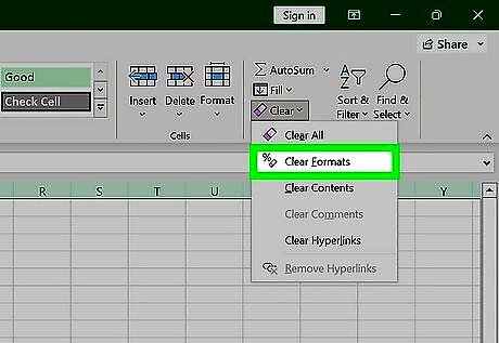
Click Clear Formats. This will clear the formatting applied to the selected cells.
Removing Conditional Formatting

Open a project in Microsoft Excel. You can use an existing project or create a new spreadsheet. When you apply conditional formatting, you're able to highlight specific cells and make them easier to identify.

Highlight the cells you want to change. You can click and drag to select the cells. To select all, press CTRL + A (Windows) or Command + A. To select a column or row, click the column or row heading. To select specific cells, hold CTRL (Windows) or Command (Mac) and click the cells you want to select.

Click Home. You can find this on the top toolbar, next to Insert. You may already be on this tab.
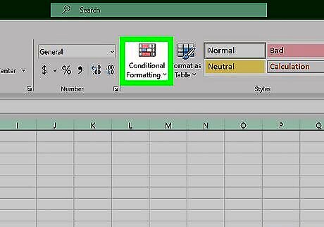
Click Conditional Formatting. A drop-down menu will open.
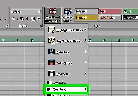
Click Clear Rules. This will expand a side menu.
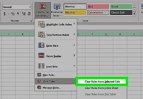
Click Clear Rules from Selected Cells. You can also click Clear Rules from Entire Sheet if you have conditional formatting for your entire Excel sheet.
Using Format Painter
Open a project in Microsoft Excel. You can use an existing project or create a new spreadsheet.
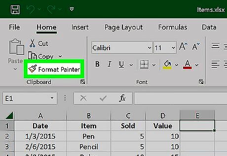
Click Format Painter. If you aren't already on your Home tab, click to open it. Format Painter will be in the Clipboard section, next to a paint brush icon.
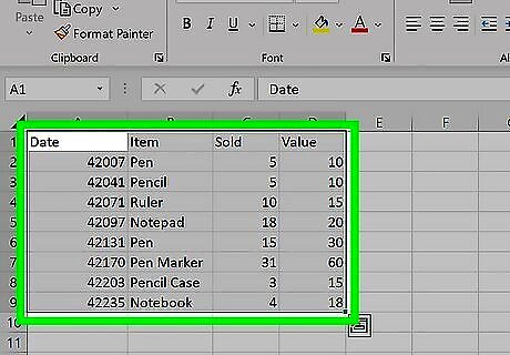
Highlight the cells you want to change. You can click and drag to select the cells. To select all, press CTRL + A (Windows) or Command + A. To select a column or row, click the column or row heading. To select specific cells, hold CTRL (Windows) or Command (Mac) and click the cells you want to select. The formatting will be cleared.
Adding Clear Formats to Quick Access

Open a project in Microsoft Excel. You can use an existing project or create a new spreadsheet.
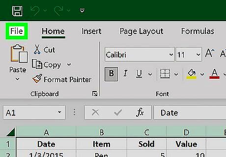
Click File. A menu will open.
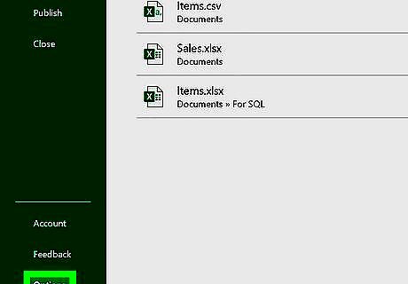
Click Options. You can find this on the left panel, at the very bottom. A new window will open.
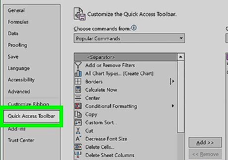
Click Quick Access Toolbar. This will be on the left panel, underneath Customize Ribbon.

Select All Commands. You'll need to click the drop-down menu underneath Choose commands from.

Click Clear Formats. You may need to scroll through the box underneath All Commands to find it. This will be next to an icon of a % and eraser.
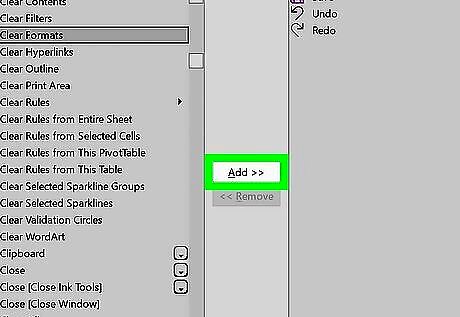
Click Add. You'll see Clear Formats in the box underneath Customize Quick Access Toolbar.

Click OK. The Clear Formats command will be added to the Quick Access Toolbar. You can find the Quick Access Toolbar at the very top, next to the Save and Undo/Redo icons.
Adding Clear Formats to the Ribbon

Open a project in Microsoft Excel. You can use an existing project or create a new spreadsheet.
Right-click the ribbon. The ribbon is the set of toolbars at the very top of the page. A pop-up window will open.
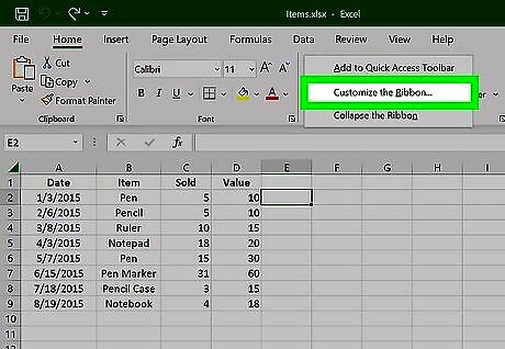
Click Customize the Ribbon…. A new window will open. You can also click File → Options → Customize Ribbon.
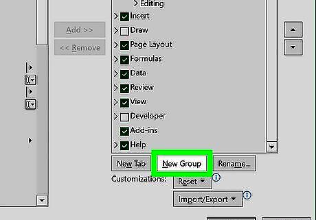
Click New Group. This can be found underneath the right box, between New Tab and Rename. Make sure to click the main tab where you would like your shortcut. This can be in Home, Insert, etc. New commands can only be added to custom groups. You can choose to rename the group by clicking Rename at the bottom of the box.
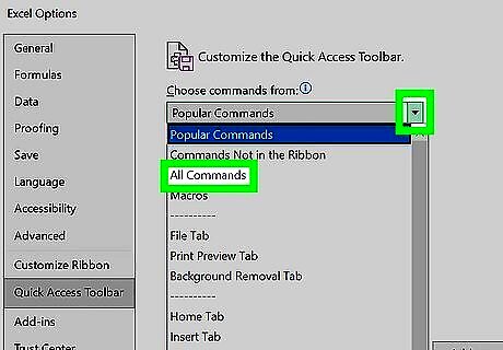
Select All Commands. You'll need to click the drop-down menu underneath Choose commands from.
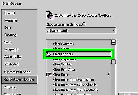
Click Clear Formats. You may need to scroll through the box underneath All Commands to find it. This will be next to an icon of a % and eraser.

Click Add. You'll see Clear Formats in the new group created below the Customize the Ribbon box.
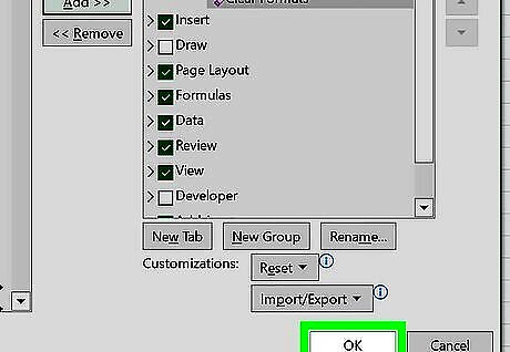
Click OK. The Clear Formats command will be added to the new group in the ribbon. Find the new Clear Formats shortcut by navigating to the tab of your new group. You'll see the new button in your ribbon.


Comments
0 comment