How to Calculate a Car Loan in Excel

Launch Microsoft Excel.

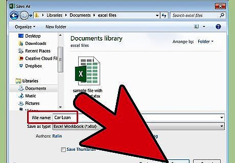
Open a new worksheet and save the file with a descriptive name such as "Car Loan."

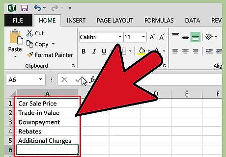
Create labels for the cells in A1 down through A6 as follows: Car sale price, Trade-in value, Down payment, Rebates, Additional charges and Amount financed.

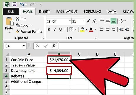
Enter the amounts for each item from your proposed car loan in cells B1 down through B5. The car sale price is negotiated with the dealership. The dealer incentive, rebates and additional features items may not apply to your situation.

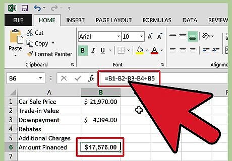
Calculate the amount financed in cell B6 by entering "=B1-B2-B3-B4+B5" in the cell, without quotation marks, and pressing "Enter."

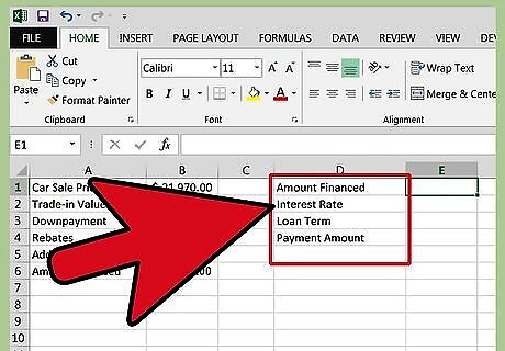
Make labels for the loan details in cells D1 down through D4 as follows: Amount financed, Interest rate, Loan Term and Payment amount.

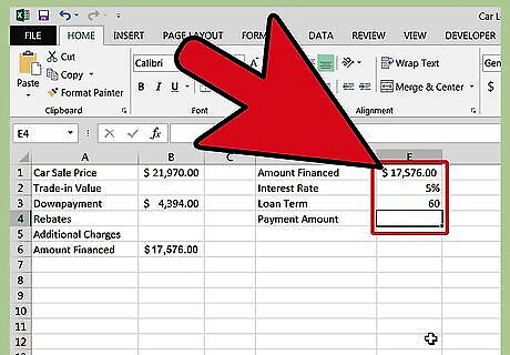
Fill in the information for the loan details in cells E1 down through E3. Type "=B6," without quotation marks, in cell E1 to copy over the amount financed. Make sure your interest rate is entered as a percentage in cell E2. Enter the loan term in months in cell E3.

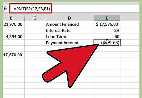
Figure the payment amount by entering the following formula, without the quotation marks, in cell E4: "=PMT(E2/12,E3,E1)."

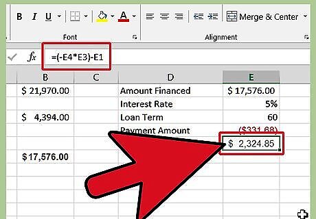
Add up the total interest paid over the life of the loan in cell E5 by entering the following formula, without quotation marks: "=(-E4*E3)-E1. In this step we must add the Amount Financed (E1) - this may seem counterintuitive, but because Excel correctly treats our calculated Payment as a cash outflow and assigns it a negative value, we must add back the Amount Financed to reach a Total Interest Paid amount." This formula calculates the total of all payments less the amount financed to arrive at the total interest paid over the life of the loan.

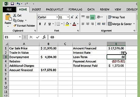
Review your entries and results and make adjustments to the variables. You can see how the scenario would look with a higher or lower interest rate, a shorter or longer loan term or with a larger down payment.