views
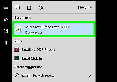
Open your Excel document. Double-click the Excel document that contains the data for which you want to use the VLOOKUP function. If you haven't yet created your document, open Excel, click Blank workbook (Windows only), and enter your data by column.
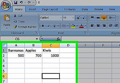
Make sure that your data is properly formatted. VLOOKUP only works with data that's organized in columns (e.g., in vertical sections), meaning that your data most likely has headers in the top row of cells but not in the far-left column of cells. If your data is organized by rows instead, you'll won't be able to use VLOOKUP to find a value.
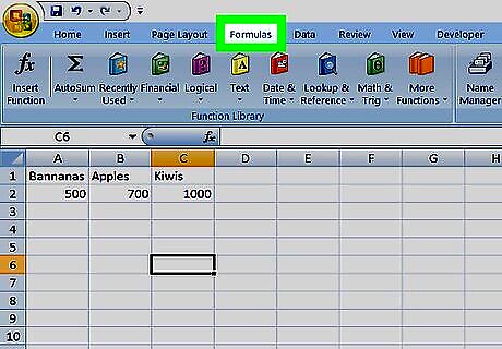
Understand each aspect of the VLOOKUP formula. The VLOOKUP formula consists of four main parts, each of which refers to a piece of information in your spreadsheet: Lookup Value - The cell across from which the data that you want to look up is in. For example, if you want to look up data in cell F3, your lookup value will be in the third row of the spreadsheet. Table Array - Your entire table's span from the top-left cell to the bottom-right cell (not including headers). For example, if your table starts at A2, goes down to A20, and extends over to the F column, your table goes from A2 to F20. Column Index Number - The index number of the column in which the value that you want to look up is in. A column's "index number" refers to its order number; for example, in a spreadsheet that has data in columns A, B, and C, the index number of A would be 1, B would be 2, and C would be 3. The index number starts at 1 for the far-left column of data, so if your data starts in column F, its index number is 1. Range Lookup - You'll normally want a precise answer for the VLOOKUP result, which can be achieved by typing in FALSE for this value. For an estimate, you can type in TRUE instead.
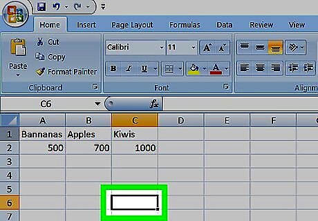
Select an empty cell. Click a cell in which you want to store the result of the VLOOKUP formula.
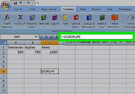
Add the VLOOKUP formula tag. Type in =VLOOKUP( to start the VLOOKUP formula. The rest of the formula will go between the open parenthesis and a closed one at the end.
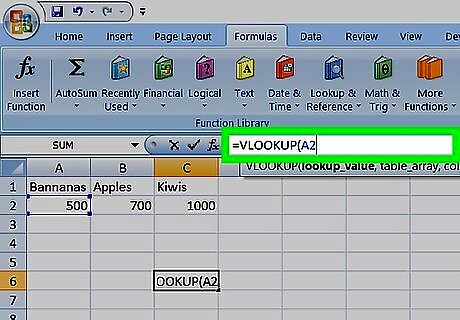
Enter the lookup value. Find the cell in which the lookup value is written, then enter the cell's name into the VLOOKUP formula followed by a comma. For example, if the lookup value is written in cell A12, you'd type A12, into the formula. You'll separate each section of the formula with a comma, but you don't need to use spaces.
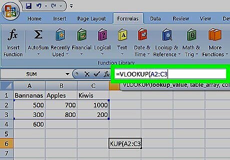
Enter the table array value. Find the top-left cell in which data is stored and enter its name into the formula, type a colon (:), find the bottom-right cell in the data group and add it to the formula, and then type a comma. For example, if your table goes from cell A2 to cell C20, you'd type A2:C20, into the VLOOKUP formula.
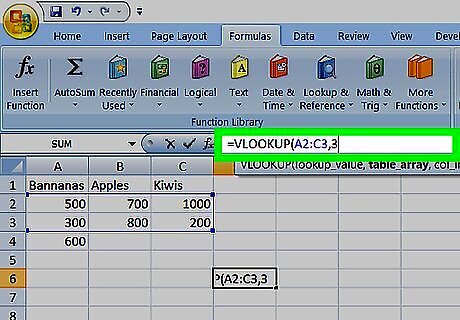
Enter the column index number. Find the index number of the column that contains the value that you want VLOOKUP to display, then type it into the formula with a comma after it. For example, if your table uses the A, B, and C columns and the data that you want is in C, you would type in 3, here.
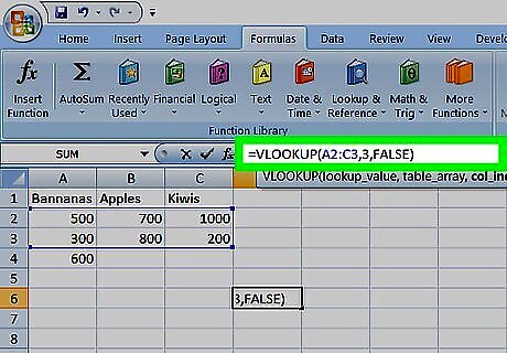
Type in FALSE) to close the formula. This will allow VLOOKUP to find the exact value in your specified column for the selected item. Your formula should look something like this: =VLOOKUP(A12,A2:C20,3,FALSE)
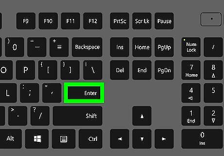
Press ↵ Enter. Doing so will run your formula and display the result in the formula's cell.


Comments
0 comment